
Introduction
Control Systems is a course I took at university previous year. I am reviewing the topics because I am currently working in this field at the company. While doing this review, I thought it might be useful to write a post about it, and I am also planning to start a series in which I will explain each field in mechanical engineering in this way. In this way, I plan to help mechanical engineering students who have difficulty in choosing a field, people who will choose a department at university, and those who take the course. Therefore, due to the audience I am addressing, I will not overwhelm with formulas that everyone can understand. I do not plan to go too far in terms of topics. However, as I work on this subject in the future, I may add separate articles.
What does a control engineer do?
The aim of control engineers is to ensure that the system operates in the desired behavior. An example of this behavior is a helicopter taking off. In this process, the pilot gives input with its collective arm, which is one of the controllers of the plane. As a result, the helicopter accelerates upward. But in this example, is the desired behavior really just to gain this take-off acceleration? In fact, this behavior can be opened much more. There are many requirements, such as how fast the helicopter reaches a steady state or how much it exceeds its steady state speed while in transient state. The aim of control engineers is to ensure that these requirements are complied with by modifying the control system and designing a controller.
Overview of Design Procedures
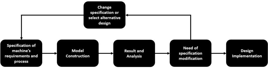
The design procedure is very important for putting theoretical knowledge into practice. If the theoretical knowledge learned is applied randomly, it is not possible to create a control system successfully. Therefore, before starting the theoretical explanation, I will talk about these design procedures and in the rest of my article, I will create this subject flow according to this procedure.
Specification of Machine's Requirements
Control systems require detailed planning before being designed. It is necessary to select the appropriate sensor for feedback systems and to evaluate the standard parameters for the system to be built. The parameters I mentioned here can be for different domains (Frequency domain, time domain). These parameters are important at the analysis stage.
Modelling Physical System
At this stage, mathematical modeling of the plant is done. The equation of each element in the system is derived and the overall transfer equation is found. Afterwards, add-ons such as the system’s controller and feedback system and sensors are placed.
Analysis of Control System
Various analysis are carried out in the 3rd stage, where the requirements of the system I mentioned before are evaluated. MATLAB or any other computational program is largely used for this stage. These analyzes vary such as steady state error analysis, stability and transient response analysis, which I will explain in the following stages. After the analysis, gain values or other unknown values that will fit the requirements are decided.
Change Specification or Select Alternative Design
The design process involves a lot of trial and error. If it is observed that the system design determined at the beginning does not meet the requirements as a result of the analysis, the controller can be changed, the system can be modified or the control type can be changed. Making all these changes and repeating the procedure can be a very tedious process, so it is very important to have an insight into what the impact of the changes will be. This requires theoretical and practical experience about control.
Basics of Control Systems
For control system design, it is very important to know control terms first. I will also show some system features at this stage to help you choose what kind of system it could be.
Components and Terms
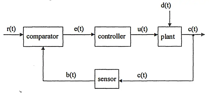
Instead of defining terms and components one by one, the example given below shows the terms we need now. However, additional explanations have been provided for some terms.
Controller
The main purpose of this device, which is the main subject of analysis and design in the control system, is to create the manipulated input in the desired state according to predetermined rules. Manual control is the situation where the controller is human. What is of interest in the field of control is automatic control, where the controller is a device.
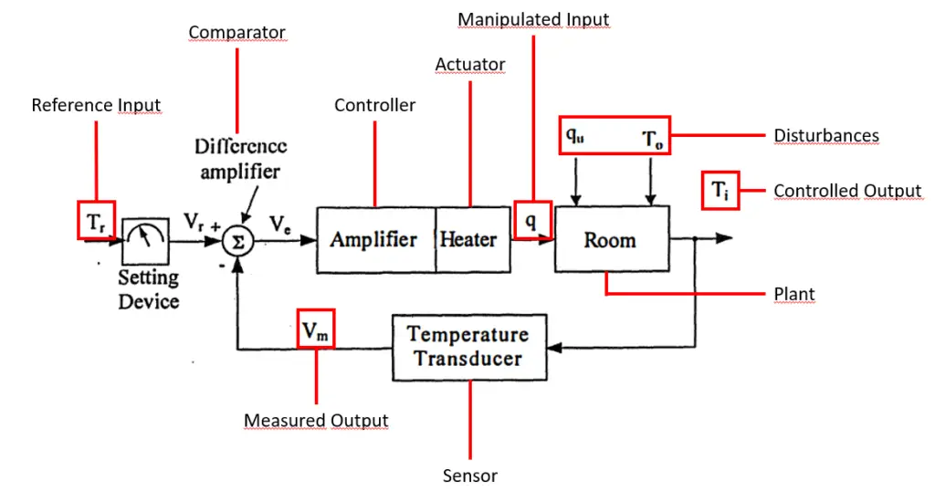
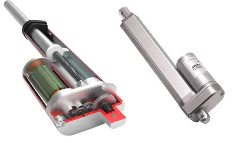
Actuator
A sensor is a device used to measure the visible output. The fact that the sensors we have are not ideal causes us to not get completely accurate results. For this reason, there is a difference between the measured output and the observed output. Additionally, another problem with sensors is the effect of disturbance called sensor noise, which is not shown in the figure above.
Types of Control
Open Loop Control
Open loop control can be thought of as a system without any sensors. For example, imagine a car and imagine that we design a controller that will allow this car to go to the desired location. Briefly, the function of this controller is to ensure that the pedal is pressed for a specified period of time and then press the brake to stop. A suitable controller is designed by establishing the relationship between this required time and distance. However, the problem here is that the vehicle cannot react appropriately to different conditions. When another vehicle is connected to the rear of the vehicle, it will take more time to get there, but the time pressed will not change. Of course, this situation can be resolved with the disturbance rejector. The primary problem for this to be done is that this disturbance is measurable. For example, an effect such as wind can be measured with sensors, but when we consider friction, there is no sensor suitable for measuring it. In addition, even if precautions are taken against a disturbance, unexpected disturbances will still cause the system to not work as expected.
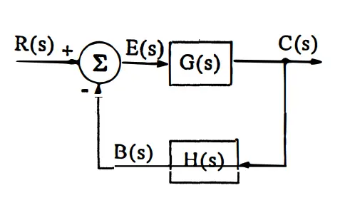
Feedback Control
A basic Feedback control system is as given above. If we continue with the previous car example, for a car using this system, disturbance will be insignificant in terms of reaching the target. The problem of such systems compared to Open loop systems lies in ensuring stability and being costly. Feedback control can be examined under two headings. These are systems where Direct FB control observed output is the same as controlled output. The example system given above is an example of these systems. Indirect FB control is a system where these two are not the same. This is mostly not a desired situation. Because it is not possible to test whether the expected situation occurs or not, and the feedback system may not fully realize the expected situation. Indirect FB control is used when measuring observed output is difficult, impossible or expensive.
Open loop and Feedback control types need to be decided when determining the requirements. You can start with OL first and return to FB control if the requirements are not met. However, it should be known that unexpected disturbances are encountered in almost every physical system. What needs to be decided is whether the system’s margin of error will be exceeded in the face of possible disturbances.
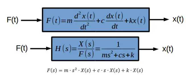
Transfer Function
The transfer function is the equation that establishes the relationship between input and output. This equation is derived by taking the Laplace transform of the differential equation. Therefore, the transfer function is defined in the s domain. Laplace transform and other details about this domain are explained in more detail in my blog post about signals and systems. In short, the reason for using the s domain is that the operations to be performed in the t domain are complex (see convolution). Obtaining a transfer function is shown below with an example.
Types of Controller
As mentioned before, the controller is the most important component designed by the control engineer for the system to work as desired. In order for the system to comply with the requirements, changes that can be made other than modifying the system are made in the controller. Apart from changing the gain on the controller, changing the type of controller is the main factor in achieving the system’s requirements. Although determining the gain is a job after the analysis, the controller type is determined at the first stage. In this section, I will separately discuss determining controllers for feedback and open loop systems.
Disturbance Rejection for Open Loop Control
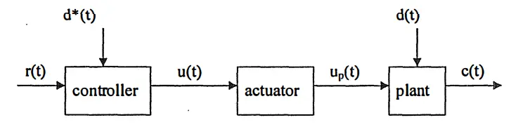
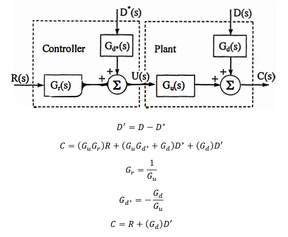
We can actually think of this heading under the heading of analyses. Since open loop systems cannot respond specifically to disturbances, it is necessary to measure or approximately calculate the disturbances and enter them as input. In this way, it is aimed to ensure that the system works as desired. However, the controller through which the reference disturbance enters the system must also be designed accordingly. Below is explained how this process is done for a typical open loop system.
As can be seen in the model given below, a controller must be designed for the plant system to operate as desired (R=C). Gd* and Gr must be determined accordingly in the controller. In order for the input and output values to be the same, Gcr = 1, Gcd * = 0 and Gcd’ = 0. However, it is impossible for Gd=0. Therefore D’ must be quite close to zero. The closer the reference disturbance given to the Controller is to the disturbance applied to the system, the more precisely the system will work.
The main reason why we can use this approach in open loop systems is actually due to the stability of open loop systems.
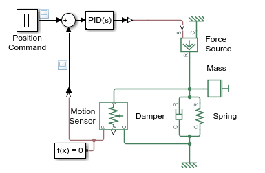
Controllers for Feedback Control
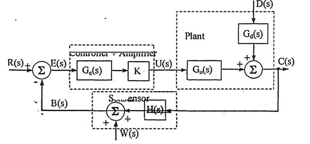
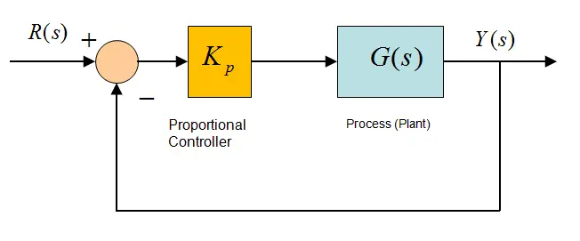
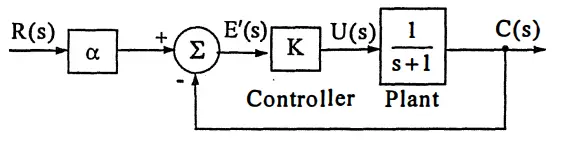
It is not possible to use the disturbance disturbance method for feedback systems, like open loop systems. This is due to the stabilization problem of feedback systems. Ready-made controller designs are preferred for feedback systems. These controllers will be explained in this section. In fact, it is possible to talk about extra controllers such as lead and lag controller, but in this article only P, PD, PI, PID controllers will be mentioned. You can see a typical feedback control system on the side. The gain calculation and the suitability of this controller will be determined during the analysis phase. What we’re deciding now is sort of deciding on the transfer function of Gc(s).
P Controller
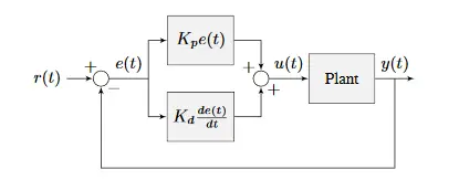
PD Controller
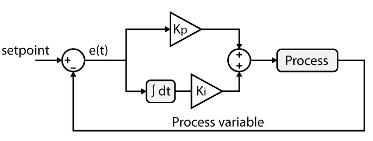
PI Controller
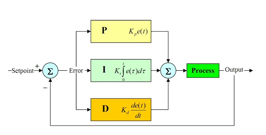
PID Controller
Modelling Physical System
To understand this stage, the first thing you need to know is that the design of the process (plant) is not what the control engineer does. Different areas make this design depending on what the system contains. For example, it may contain plant thermal, fluid flow, mechanic and electronic components. In order to design this system, it is necessary to work together with each field. Modeling using the equations in this designed system must be done by the control engineer. System modeling consists only of formulas, so it does not make sense to examine each component in depth right now. Below are examples for fluid, thermal, mechanic and electrical systems. If you want more details about the modeling phase of these systems, you can find them in the resources I will give in the references.
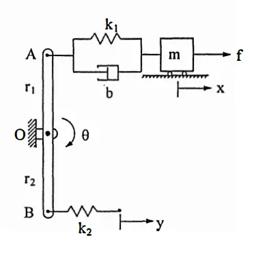
Mechanical System
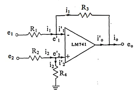
Electrical System
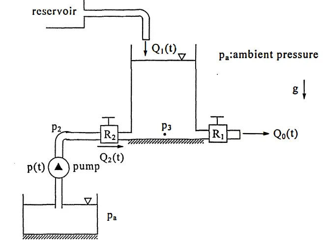
Fluid System
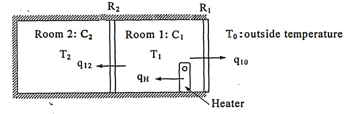
Thermal System
Analysis
Before starting this stage, let’s first go over what we have completed so far. First of all, we decided on the type of controller, actuator and control type of the control system we will make. The requirements of the system were decided. Afterwards, the physical modeling of the system for the plant was completed. Now we will analyze the system and try to ensure its compliance with the requirements. If this is not possible, changes will be made and the steps will be repeated. The analyzes to be explained in this article will be stability, steady state response and error and transient response, respectively. I should point out that frequency response analysis is also very important for control. However, since I think my knowledge about them is not sufficient, I will only focus on these 3 analyzes for now. I am planning an article in the future where I will talk about it.
Stability
Stability can be briefly defined as whether the system will return to its initial equilibrium position after input is given to the system. For this analysis, it is assumed that impulse input is given to the system. In other words, impulse response is examined. What needs to be examined for stability analysis are the poles (making undefined) and zeros (resetting) the transfer function of the system. The stability behavior of the system can be understood according to their positioning on the complex surface. The stability behavior of the system can be divided into 3, these behaviors are explained below.
Asymptotic Stability
t → ∞, [y(t), g(t)] → 0
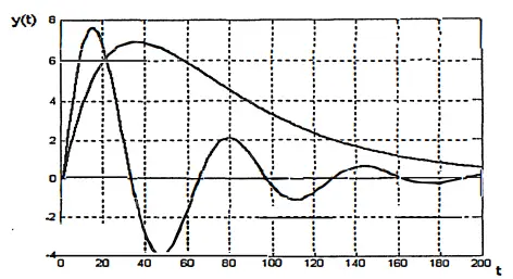
Asymptotic stability, also known as stable system output, returns to its previous state after any input. The graph below explains this situation. A stable system occurs when all poles of the transfer function have negative real parts.
Marginal Stability
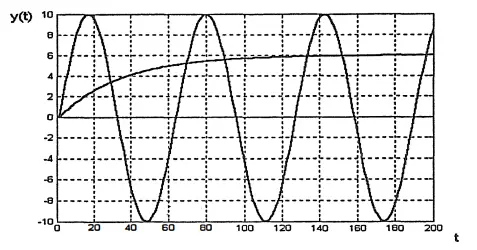
t >0, |g(t)| < b < ∞
Marginally stable systems occur when the system does not reach 0 after impulse input is given, but remains within a certain range. This is possible if the transfer function has a pole whose real part is 0 and does not repeat. Apart from this, the system should not have poles with positive real parts.
Instability
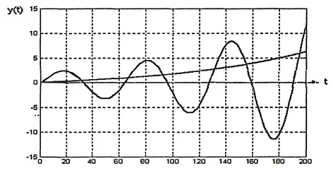
If the transfer function has a repeating pole on its imaginary axis or a pole on the positive real axis, then the system is not stable.
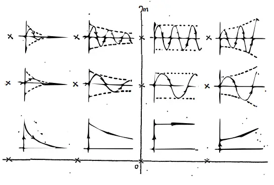
Depending on the requirements of the system, different gain ranges are obtained for stable, marginally stable or unstable. Below you can see an example of a graphic obtained as a result of the analysis. In addition, a graph of how the system will behave according to the pole positioning is also given. While the stability of the system can be checked according to pole positioning, this process is quite difficult for high-order equations. Therefore, different methods have been developed for stability analysis. Routh-Hurwitz Criterion is one of the stability analysis methods that we frequently use in class. But I don’t think I’ll go into details right now.

Steady State Error Analysis
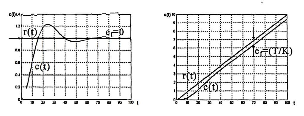
In Steady State Error Analysis, as the name suggests, the error (e(t), E(s)) that occurs when the system reaches steady state is dealt with. For this purpose, the E/R transfer function is written. As expected, the error varies depending on the type of input (impulse, ramp, step, acceleration). The chart below shows how the error changes depending on the input. Additionally, two different graphs are given to understand what the error is.
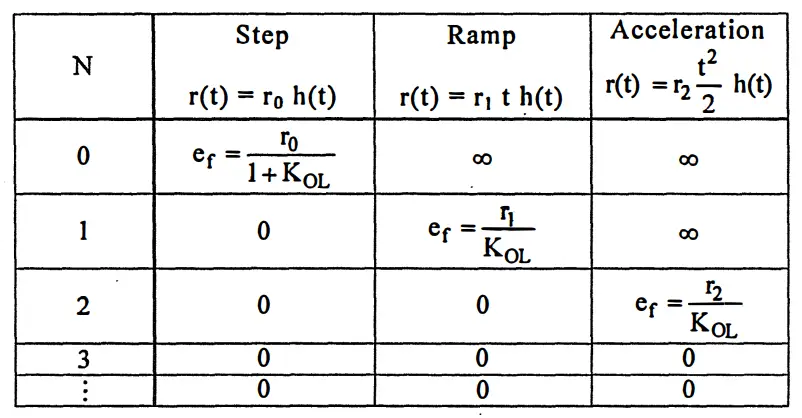
As can be understood from the table showing the error and input relationship, the type number may need to be increased in order for the error in the system to converge or remain constant. To achieve this, the system must be modified. 3 different modifications are mentioned below. If the initially created system does not meet SS error expectations, one of these modifications must be made. First of all, replacing the controller with a PI controller is not a frequently used modification. Because it increases the order of the system. Compared to this, it is recommended to use the other two methods more frequently. In these two methods, the coefficients added to the system must be precisely adjusted. I have briefly mentioned the details of this exact adjustment process below, but I will not go into the process.
PI Control
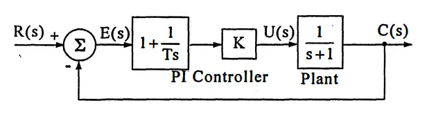
Adding the PI controller to the system will increase the type number and thus eliminate the SS error in the system.
Modified Reference
When such a modification is made, it is necessary to find the transfer function of the system, model the system as the initial state we gave at the beginning of the topic, and find the corresponding open loop transfer function. Afterwards, it is necessary to determine the new coefficient in the system in a way that will increase the type number, that is, make the coefficient in front of the variable with the lowest order in the transfer function zero.
Feedforward Contribution
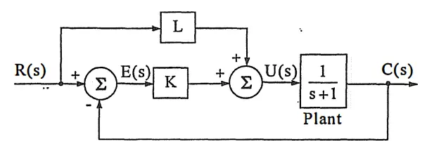
Feedforward Contribution is determined by the same method as Modified reference.
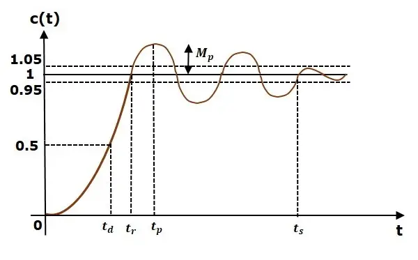
Transient Response
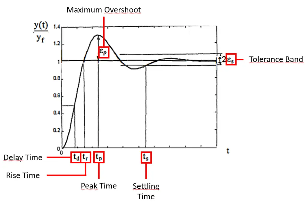
Transient Response is related to the behavior of the system before it reaches steady state. The parameters to be determined for this behavior can be examined under two headings. Firstly, the speed at which the system reaches SS and secondly, the relative stability of the system, which is related to the fluctuation and overshoot behavior of the system. You can see the parameters related to these behaviors in the graph on the side. After classifying the behavior of the system we will make at this stage (This classification is not explained in this post. In short, finding out whether the system is first-order or second-order and then determining what behavior it shows, such as overdamped, underdamped, etc.), gain or other parameters are found to comply with the determined standards.
Conclusion
In this post, I tried to show what a control engineer does in a process by explaining the basics of control systems and system design. However, I had to skip some topics because explaining them required entering into formulas or because it was too long for this article. Also, I only mentioned the analyzes for the time domain. Since even that would make it too long, I have only gone superficially. Since I will be working in this field at the moment, I will try to close all these deficiencies with additional posts. However, since the main purpose of this post is to help engineer candidates who want to choose a field and to help someone who does not know anything about the basics, I do not think it will meet the expectations. Don’t forget to follow me for more advanced information or such articles in different fields.
References
- ME 304 Lecture Notes
- Katsuhiko Ogata, Modern Control Engineering, Fifth Edition