
Finite Element Analysis Project
ME 308
FEM
C++
Latex
2024
Deal.ii
Heat Transfer
About Project
In this project, four different heat transfer problems were analyzed using the Finite Element Method (FEM). The first problem involved solving and modeling a 2D steady-state heat transfer problem in a half-annular shape. The second problem focused on a 2D steady-state heat transfer problem in a chip with fins. For the third problem, the same structure as the second problem was considered, but with the assumption of free convection. In the final problem, the structure from the second problem was modeled in 3D and the 3D steady-state heat transfer problem was solved.
The theoretical solutions included derivations for the weak formulation, the creation of elemental matrices, the assembly of these matrices into a global matrix, and the assumptions made to determine the boundary conditions. Detailed reports were provided on how we manipulated the matrix problem using these boundary conditions to make it solvable.
All problems were solved using the deal.ii library with C++, ensuring rapid problem-solving. By leveraging deal.ii’s features, such as adaptive mesh refinement and sparse matrices, we achieved more accurate results and reduced the memory requirements for the matrix. The memory load of classical matrices versus sparse matrices was calculated and reported. Additionally, results from numerical integration with different orders were documented. Through these efforts, we have comprehensively addressed the solution of FEM problems both theoretically and practically.
I have organized the project into detailed segments for each part, and you can find further details at the bottom of the page. I took responsibility for preparing the project’s foundation, implementing adaptive mesh refinement in the first part, and conducting memory measurements. Other team members wrote code for adaptive mesh refinement and runtime measurement for the remaining parts. The project’s report was completed individually.
FEM
The Finite Element Method (FEM) is a numerical technique for solving complex engineering and mathematical problems. It is widely used in various fields such as structural analysis, heat transfer, fluid dynamics, and electromagnetism. FEM works by breaking down a large, complex problem into smaller, simpler parts called finite elements. These elements are connected at points called nodes, and the solution is formulated by creating a system of equations based on the physical laws governing the problem.
One of the key advantages of FEM is its ability to handle irregular geometries and complex boundary conditions with high accuracy. This flexibility makes it a powerful tool for engineers and scientists to model and simulate real-world scenarios, providing insights and solutions that would be difficult or impossible to achieve with traditional analytical methods. By using FEM, one can optimize designs, predict performance, and ensure the reliability and safety of various systems and structures.
Deal ii
Deal.II is a powerful, open-source C++ software library designed for solving partial differential equations (PDEs) using the finite element method (FEM). It provides a comprehensive framework for developing finite element codes, making it accessible for both beginners and advanced users in scientific computing.
The library supports a wide range of finite element methods and offers features such as adaptive mesh refinement, support for complex geometries, and efficient handling of large sparse matrices. These capabilities enable users to tackle complex, real-world problems with high accuracy and efficiency.
Deal.II is actively maintained and continuously updated, with extensive documentation and a vibrant user community. It integrates well with other scientific computing libraries, offering a robust platform for research and development in computational science and engineering.
Steps of Each Part
- Define the problem geometry and boundary conditions.
- Perform weak formulation of the governing equations.
- Construct elemental matrices using the shape functions.
- Assemble the global matrices from the elemental matrices.
- Apply boundary conditions to modify the global matrices.
- Implement the solution algorithm using the deal.ii library in C++.
- Solve the matrix equations to obtain the temperature distribution.
- Perform adaptive mesh refinement for improved accuracy.
- Compare results with different numerical integration orders.
- Analyze the memory requirements for classical vs. sparse matrices.
- Discuss and document the results and findings.
Conclusion
In this project, we successfully analyzed four different heat transfer problems using the Finite Element Method (FEM) and the deal.ii library. By solving 2D and 3D steady-state heat transfer problems, both with and without convection, we demonstrated the versatility and power of FEM in handling complex geometries and boundary conditions. The implementation of adaptive mesh refinement and sparse matrices significantly improved the accuracy and efficiency of our solutions.
Throughout this project, we had the opportunity to apply the concepts learned in our ME 413 course, enhancing our theoretical understanding and gaining practical experience in using advanced computational techniques. This comprehensive approach allowed us to effectively tackle real-world problems and reinforced the value of FEM in engineering analysis.
Part 1
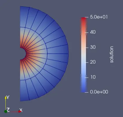
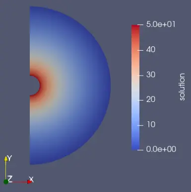
In this part of the project, we will analyze a half-annulus-shaped geometry. The equation governing the heat transfer and the boundary conditions are defined in the problem statement, with Figure 1 illustrating the geometry and boundary conditions. Initially, we perform the weak formulation of the partial differential equations. Subsequently, we construct the Jacobian matrix to define the right-hand side (RHS) and left-hand side (LHS) matrices. After generating the elemental coefficient matrices, we assemble these matrices. Prior to solving the matrix equation, boundary conditions are applied. In the implementation and improvement section, we provide a brief explanation of the code and suggest enhancements to improve the efficiency of the solution process. The results section presents all findings related to this problem.
Discussion
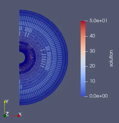
In this part of the project, we used the given heat transfer equation to determine the temperature distribution within a half annulus shape. Initially, we demonstrated the numerical procedures to obtain the weak formulation of the equation. We then discussed how this equation can be theoretically solved using quadrilateral elements. By defining the boundary conditions, we showed how we adjusted the assembled global matrices. Using the weak formulation and boundary conditions, we developed a program to solve the system. To refine the meshes and reduce discontinuities, we used mesh refinement techniques. Additionally, to enhance the speed of the program, we employed sparse matrices, observing a performance increase of up to nine times compared to traditional matrix solutions. The implementation of sparse matrices was more straightforward thanks to deal.II’s native support. Classical matrix method store lots of zero due to behaviour of FEM. While solving FEM problem. In the matrix, there are lots of zeros and generally it is diagonal. Storage of these large number of zeros will be a trouble for computer and lead to collapse. As seen in the table there is a huge memory difference.
We also examined how the system behaves with different Gauss quadrature orders and presented the results in tabular form. As expected, increasing the integration order raised the computational cost, but beyond a certain point, the error rate in the calculations remained unchanged. This invariance can be seen from the active cell count, which stayed the same for higher-order computations. Finally, our graphs indicated that adaptive mesh refinement assesses the error for each mesh and introduces additional meshes where the error exceeds a threshold. This results in a more accurate temperature distribution. Initially, some gaps appeared between adjacent meshes due to the refinement process, but these diminished significantly after a few cycles. For further accuracy, increasing the cycle count may be necessary, which also requires adjusting the maximum iteration count in the solve function. We concluded our refinement at a point where we believed the results were sufficiently accurate, thereby saving time in testing various conditions.
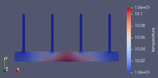
Part 2
In this section, we will examine a silicon chip and its cooling mechanism, which involves copper fins. To simplify the problem, we will reduce the normally three-dimensional structure to a two-dimensional model. Our approach assumes that the temperature within the fins is constant and equal to the temperature of the surrounding water, with the copper placed on an insulated bed.
Initially, we will derive the weak form of the heat transfer equation. The theoretical framework for constructing the right-hand side (RHS) and left-hand side (LHS) matrices will be outlined, similar to the steps taken in Part 1. Next, we will delve into the boundary conditions and our approach in greater detail, demonstrating how these conditions manipulate the global matrices to make the system solvable.
Following this, we will explain the code developed to solve the problem, highlighting the improvements made to enhance its performance. The results obtained from the code, including temperature distribution graphs, outcomes from different integral orders, and results from various matrix-solving algorithms, will be presented in the Results section. Finally, we will evaluate these results and discuss their implications.
Discussion
Boundary conditions were defined and manipulated, integrating mesh refinement for accuracy. Using sparse matrices enhanced computational efficiency significantly, achieving nearly a 20-fold speed increase compared to traditional methods, leveraging deal.II’s native support for sparse matrices.
We explored different Gauss quadrature orders, finding that an integration order of 3 sufficed without significant differences observed at higher orders, guiding subsequent problem analyses.
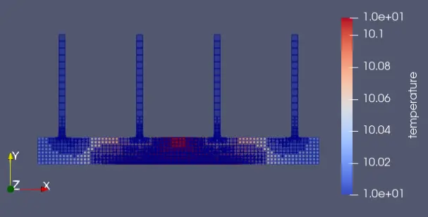
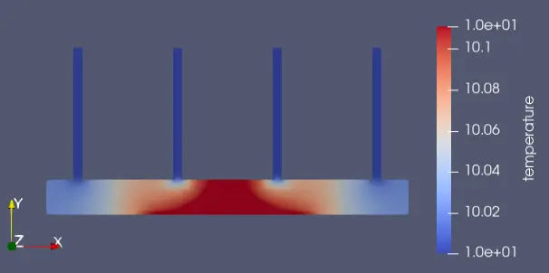
Part 3
In this part of the project, we continue analyzing the same 2D geometry as in Part 2. However, instead of assuming the surface temperature of the fins is equal to the water temperature, we will consider the assumption of free convection. This approach requires an additional iterative process, which will be detailed in the boundary condition section. Once the surface temperature is determined, adjusting the temperature values in our code will provide the desired results.
Discussion
This section follows the methodology established in Part 2 but introduces the critical task of independently determining boundary conditions. Our main focus was identifying the necessary assumptions and equations for accurate modeling.
The initial assumption for boundary conditions was that all surfaces, except fin surfaces, were insulated, similar to Part 2. For fins, we assumed free convection conditions.
To incorporate free convection, we initially assumed constant temperature along fin surfaces. Using free convection equations and fluid properties, we iteratively determined surface temperatures, detailed in the boundary conditions section.
Before implementation, we derived the weak formulation of the heat transfer equation, ensuring consistency with our prior work. This formulation guided our implementation in deal.II, mirroring the process from Part 2.
After coding and describing enhancements, we presented results, including graphical temperature distributions. Results closely resembled those from Part 2. Increasing cycles in adaptive mesh refinement significantly altered discontinuity regions and overall temperature distribution, underscoring the need for iterative accuracy.
While specific values changed, the temperature difference remained constant, yielding similar observations and conclusions to Part 2. For deeper insights, referring to Part 2’s discussion is recommended.
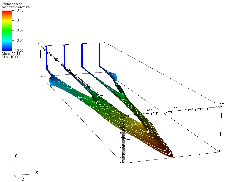
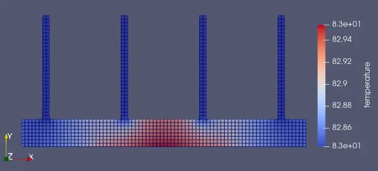
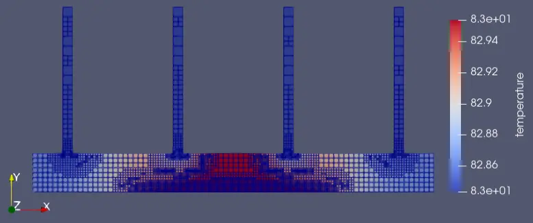
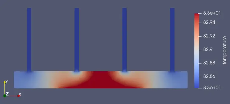
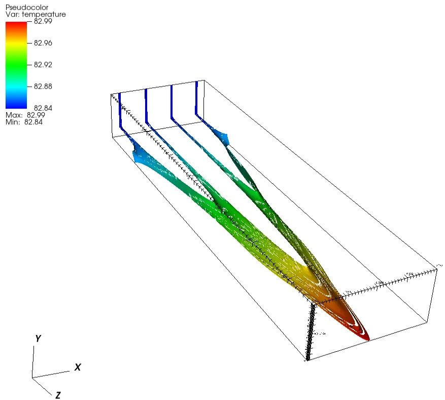
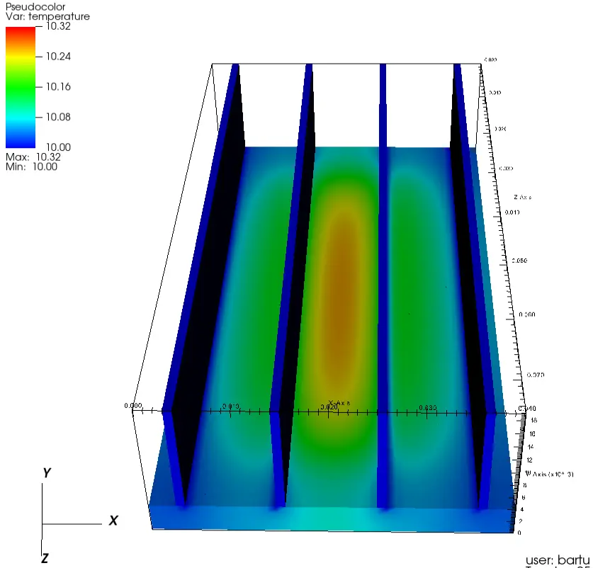
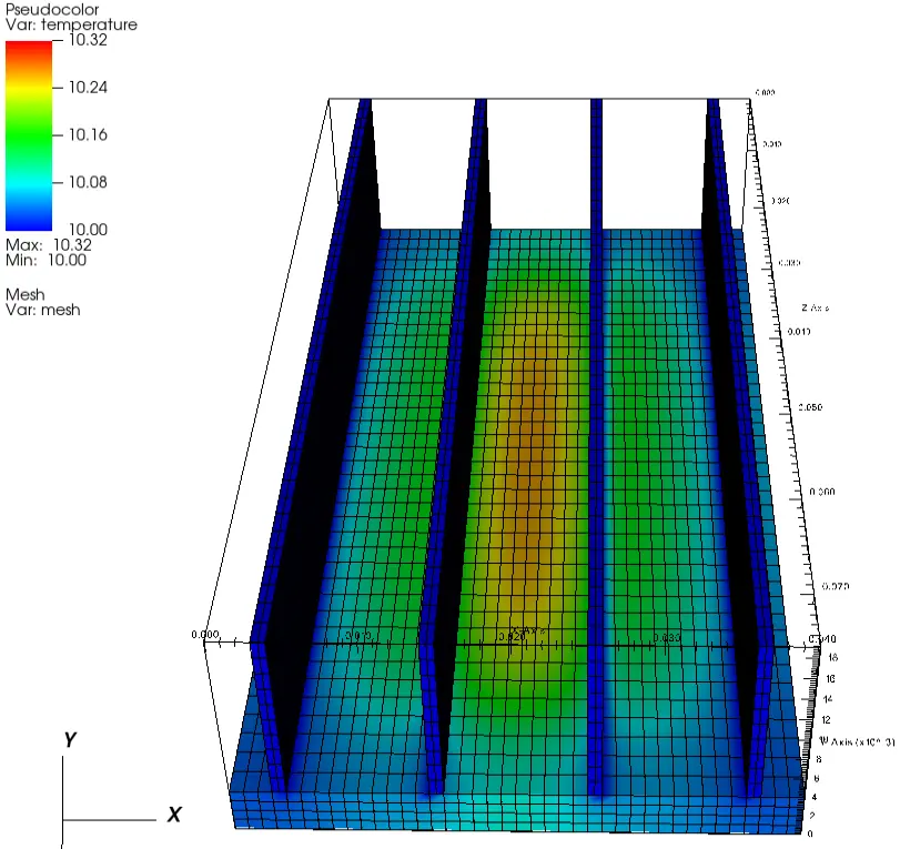
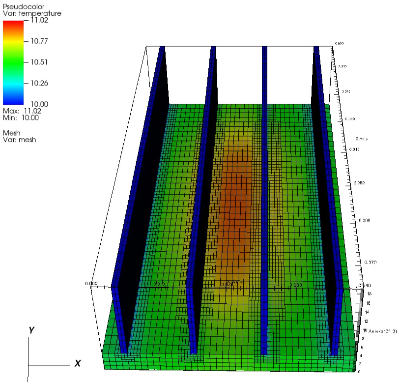
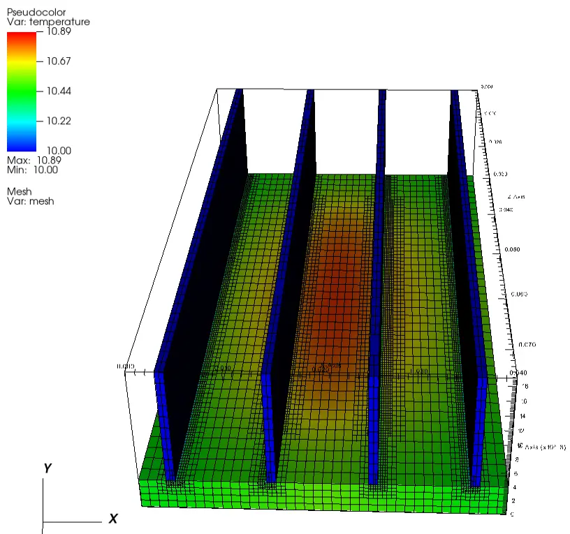
Part 4
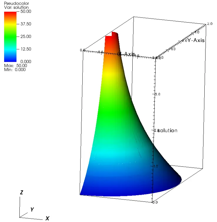
In this part, we extend the analysis from Part 2 to a three-dimensional steady-state solution. Adding the z-axis alters the weak formulation and the construction of the elemental matrix. Although the weak formulation will be derived, the elemental matrix will not be explicitly solved in this section. The shape functions now need to be defined for the eight corners of the cube, resulting in eight shape functions. Additionally, the Jacobian matrix will include the extra z-axis, complicating its computation.
Despite these changes, the overall process remains similar. After deriving the weak formulation, we will define the boundary conditions. Since this system follows the same approach as the 2D system, the boundary conditions will be largely similar. In the implementation section, we will discuss how the code differs from the 2D version. Following the solution of the problem, the resulting graphs will be presented, and the details of the problem will be discussed.
Discussion
In this part, we extended our study to the 3D steady-state heat transfer problem using the geometry defined in Part 2. Introducing the z-axis impacted both the weak formulation and the elemental matrix construction. While we solved the weak formulation, we didn’t delve into the detailed derivation of the elemental matrix. The shape functions were redefined to accommodate the eight corners of a cube, resulting in eight shape functions. The Jacobian matrix now includes the z-axis, adding complexity beyond the increased number of shape functions, though the overall process remained similar.
After formulating the weak problem, we defined boundary conditions. The approach mirrored that of the 2D system, making the boundary conditions largely similar. In the implementation section, we discussed modifications and enhancements to our code originally designed for the 2D problem. Deal.II’s capabilities made defining and meshing 3D shapes straightforward.
We applied adaptive mesh refinement as in previous parts. However, due to increased mesh complexity in 3D shapes, computation time significantly increased with each cycle, sometimes taking days. Therefore, we limited cycles to two after the initial meshing. Post-adaptive mesh refinement graphics exhibited notable issues: maximum temperature increased with mesh complexity, and significant anomalies appeared in temperature distribution. Despite attempts to address this using refined grid subclasses, issues persisted. While further cycles might resolve these, extended computation times make this impractical. Initially longer, computation times were reduced by decreasing mesh count and quadrature values, resulting in rectangular prism mesh shapes instead of cubes.