
Introduction
Finite Element Analysis (FEA) was a course I took during the 2023-2024 spring semester. With the term just ending and the topic fresh in my mind, I decided to prepare this blog post. This also marks my return to blogging after a long hiatus. At our university, the FEM course focuses on structural applications in the fall semester and on heat and fluid applications in the spring. While much of the content is similar, please note that my primary interest lies in the heat-fluid area.
This post will cover the 1D FEM formulation. I will discuss what FEM is, the concept of weak formulation, what Galerkin FEM entails, the extraction of elemental matrices, the assembly process, and the application of boundary conditions. During the semester, I completed two assignments on these topics, which I recommend checking out as examples. In future posts, I plan to delve into transient and 2D FEM formulations. By doing so, I aim to cover most of the concepts we learned throughout the semester.
What is Finite Element Method?
The Finite Element Method (FEM) is a numerical technique that allows for the solution of differential equations that are difficult or impossible to solve analytically. This enables the solution of these equations for complex geometries. It works by dividing the complex structure into finite elements, called a mesh. Each element is analyzed under specific boundary conditions, and the behavior of the entire system is determined by assembling these individual element solutions. The ability to solve complex problems easily has led to its use in many fields, including heat transfer, structural analysis, fluid dynamics, electromagnetic analysis, and even manufacturing.
Although FEM simplifies problems to a level that can be solved manually, the increase in the number of mesh elements and thus the size of the resulting matrix has led to the development of numerous software tools in this field. Common FEM software includes ANSYS, Abaqus, COMSOL Multiphysics, SolidWorks Simulation, Altair HyperWorks, OpenFOAM, and CalculiX. These tools provide comprehensive solutions for various FEM applications, catering to the specific needs of different industries.
Weak Formulation
Now, let’s begin our FEM solution by converting our differential equation into its weak form. The purpose of obtaining the weak form is to reduce order of differential equation. In addition, weak form naturally incorporates boundary conditions, particularly the natural (Neumann) boundary conditions. Essential (Dirichlet) boundary conditions are usually imposed separately. At the boundary condition part, more details can be found.
Test function is a arbitrary function. It will be used for reduce integral order as explained above part which weak formulation purpose is explained. Now, turn back our weak formulation, integrating both side of equation and multiplying with test function, our equation become:
Do you remember integration by part? Now, we will use it in order to get rid of second order differential equation. First equation given below show integration by part. Second one is obtained from combining previous equation with integration by part equation.
Above equation is weak form of our differential equation. Now, we should make approximation to solve this equation and define shape function.
Approximate Solution and Shape Function
As understandable, we try to obtain approximate solution for u function. In order to solve weak formulation, u is approximated as following. u_i means solution of u at assigned point and S_i is shape function. It will be explained.
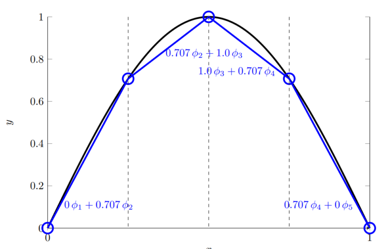
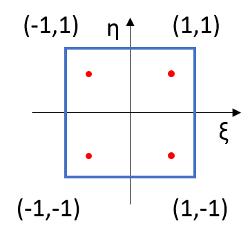
Here, k is number of element. On the right figure, shape functions are defined. Phi terms can be thought as shape function (S). Actually, shape function can be different than this. Higher order shape functions are possible. If 2nd order polynomial is selected, shape function defined with 3 point.
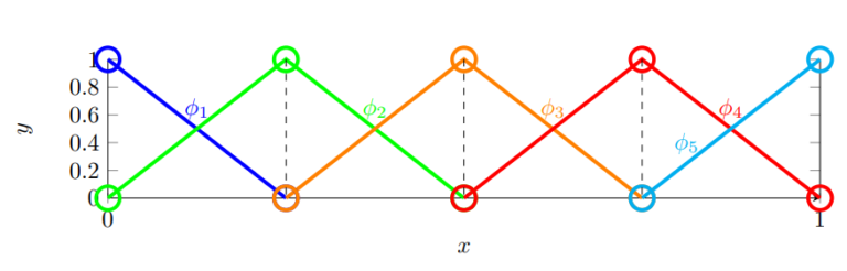
As a general equation, number of point needed for shape function M = N+1 (M is number of point and N is order). Shape functions are one at associated point and for others it is zero. More details about higher order elements will be discussed at another post. Now, we need to equate shape function. Before that, mapping process should be explained.
Mapping
Mapping means changing domain. In 1D, mapping process is x \to \xi. Shape function is defined for the mapped coordinates also. This mapping process is needed for gauss quadrature integration. This numerical integration method will be explained at further parts. For this mapping process, x and S can be defined as:
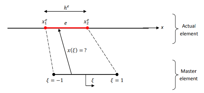
At that point, we should determine test function. In Galerkin FEM approach, w = S_i. With all these formulas, we are ready to construct elemental matrices. Note that, h means element size as seen in the figure.
Elemental Matrices
Using previous formulas and combining them, we obtain:
This equation can be written as matrix equation as [K]\{u\} =\{ F \} +\{ B \}. K is stiffness matrix, F is force vector and B is boundary integral vector. Note that it is global matrix equation. We can construct elemental matrix for each element, and then, assembly them to obtain global matrix equation. For the following process firstly LHS elemental matrix will be solved.
Elemental Stiffness Matrix
Note that d\Omega = dx for this problem that means d\Omega= \frac{dx}{d\xi}d\xi. For each element \xi is defined between -1 to 1. Our elemental stiffness matrix become:
We know all variables and parameters. It gives 2×2 matrix after solve integration. Now, let’s see how this integration will be solved. Solution won’t be done of this integration because it is long expression to put here.
Gauss Quadrature
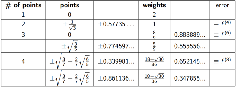
While solving integration, we will use computer, so we need a numerical integration method. Gauss quadrature is a simple and power numerical method for integration. If order of polynomial expression is known, then error can be reduced to zero. In order to apply gauss quadrature integration should between -1 to 1. Otherwise, another mapping type operation is needed. It will complicate integration. However, for our case integral is between -1 to 1. Simply, we can use gauss quadrature.
Weight values, and points are needed as seen from the function. Below these data and error of integral is given also. For example, for 4th order gauss quadrature 2 point is enough for exact solution. Also, visual mean of gauss quadrature is given in the following figure.
Elemental Force Vector
Constructing elemental force vector is similar with elemental stiffness matrix. After combining all functions above, we obtain following equation. Integration will be done with gauss quadrature again.
Elemental Force vector is as given. Although elemental stiffness is not given it is similar either. Now, we can obtain global matrices after assembly process.
Assembly
Elemental matrices are constructed above. In order to assembly each elements together, simply sum each matrices. Following two equation explain assembly process for stiffness matrix and force vector respectively. “N” is total number of elements.
Boundary Conditions
Derivations for Boundary Conditions
In order to matrix equation is solvable (unique), we need boundary conditions. As you can see from following boundary condition matrix we need to define 2 boundary conditions. One for starting side, one for ending side. Actually for 2D FEM equation or 3D, it is similar too. We should define boundary conditions for outer meshes because inner meshes are not boundary. In addition, remember shape function is one for assigned point otherwise it is zero. This property is used in second equation which is given below.
There are two type of boundary condition exist. One of the is essential BC. It is used when exact value of function is known. Natural BC is used when derivative term is known. For essential BC, matrix manipulation is needed. This manipulation is shown in following equations.
Applying Boundary Conditions
For normal BC, we should use above equation and start matrix calculation. However, if there is any essential type BC exist, then some modifications on RHS vector and LHS matrix should be applied. LHS matrix means stiffness matrix, RHS vector is sum of force and Boundary condition vector. At below, this process is shown. As expected, RHS matrix associated to that element equal to exact value, and associated value at LHS is 1 and others are 0. Equation give below helps to understand this procedure.
Solving Matrix Equation
Matrix equation can be expressed as above for two side essential BC’s. After this point, we should solve matrix equation. Gauss elimination is one of the option. However, as you can see our matrix is diagonal, so it does not a good option for memory and response speed. Thomas algorithm can be considered at that point. It gives fast response. In addition, usage of sparse matrix is a good option to construct matrix. With sparse matrix, it won’t store zeros so it has positive affect to memory. In this post, details of them will not be given. Just as a advice it is written.
Example
As a short example, let’s solve 1D heat transfer equation which is given above and boundary conditions for two sides are defined. In order to solve equation easily, equal sized two elements will be used. Constants are known and given as u = 3, k = 1, f = 1. T_1 = 0^oC and T_3 = 0 ^oC. Also x is defined from 0 to 1.
Weak formulation of similar differential equation is done at previous parts. Using that formula with some modifications, elemental stiffness matrices is obtained as following:
Note that, actually \frac{dx}{d\xi} term is jacobian. In 2D, it will be our primary challenge. However, 1D has just one parameter, so defining it is easy task. In order to avoid complexity of this post, it is not explained. It will be defined at 2D FEM post. Now, turn back our problem. In this problem, 2 element is used so each element size is h=0.5
With all of these equations, we can calculate elemental matrix. Let’s calculate elemental stiffness matrices seperately.
Between two elements, at elemental stiffness matrices, all constants and variables are same, don’t need to calculate that. If we select different step sizes for these two element, it should be calculated again. Also, if source function not constant and depend on x, again, it should be calculated. However, for this question, won’t be needed. As a result, elemental matrix and global stiffness matrix are given as following.
Let’s deal with force vector. As previous one, derivations are started from elemental matrices.
In this question we have essential type boundary conditions. Actually, there is no need to define boundary condition vector for this condition. However, let’s construct it. As before, lets continue from where we left.
All parts of matrix equations are derived. Matrix equation can be written as follows. However, boundary conditions are essential type. we need to manipulate matrix equation. After application of boundary condition, we obtained matrix equation as second equation.
After solving this matrix equation, temperature value are found as follow:
Conclusion
In this blog post, I have discussed how we can use the Finite Element Method (FEM) to solve problems that are either impossible or difficult to solve analytically in our daily lives. This introductory article on FEM focuses on solving 1D FEM problems. However, it is crucial for providing the background necessary for higher-dimensional problems. Rather than focusing on practical applications, I aimed to establish the theoretical foundation of FEM.
I have provided all the necessary formulations for solving FEM problems with explanatory details. As described in my post, solving an FEM problem involves several steps: weak formulation, creation of elemental matrices, assembly implementation, and application of boundary conditions. I also discussed some commonly used numerical approximations. This approach is intended to facilitate the preparation of an FEM program.
At the end of this comprehensive discussion, I included an example to clarify any remaining questions. By preparing this post, I have documented the concepts I learned during the FEM course for future reference and shared my knowledge of FEM with you, my readers. While this post may be challenging for the general audience, I believe it serves as a useful introduction to FEM for those with a mathematical background. Additionally, you can find my assignment files below, which I hope will be helpful.
References
- Sert, C. ME582 Lecture Notes. Middle East Technical University, Department of Mechanical Engineering.
- Baran, Ö. U. ME413 Lecture Notes. Middle East Technical University, Department of Mechanical Engineering.