Bartu Kurtulus

2D Finite Element Analysis

Introduction

We continue our FEM series with 2D in this post. However, you can also consider this content as applicable to higher dimensions. There is no need for a separate content for 3D FEM as all the fundamentals are laid out here. Adjusting the shape functions will suffice to transition to 3D. Detailed information about shape functions will be provided in subsequent posts. This content will not delve into the topics covered in 1D FEM as much, so I recommend starting with that. The reason for preparing these posts is to reach those who need them for the course I took during the semester and to create a document that I can refer to later.

In this blog post, we will sequentially reduce the order of the partial differential equation with weak formulation, discuss the Jacobian matrix, and connect this topic with 1D FEM. After that, we will form our elemental matrices, perform assembly to obtain global matrices, and briefly talk about boundary conditions. Finally, we will solve an example problem to better understand the topic. Homework assignments I completed for the course are also provided. So, let’s get started with the content.

FEM in Higher Dimensions

In the previous post, we discussed 1D FEM; however, FEM applications are predominantly carried out in 3D or simplified to 2D. Although similar procedures are followed, some aspects need further elaboration. Various changes occur in Gauss Quadrature and the Jacobian matrix, increasing the complexity of the problem. Additionally, as the dimension increases, the number of required meshes and consequently, the size of the matrices used in the problem also grows.

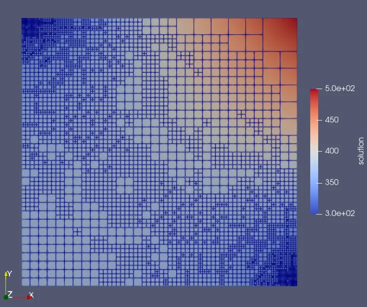
This necessitates the use of various algorithms to make computational solutions feasible, such as using sparse matrices to reduce memory requirements and distributing the load on the processor using multicore systems. Libraries used in the FEM field especially support these algorithms. For example, I use the deal.ii library, which allows for implementing the problem and refining the results using adaptive mesh refinement to eliminate errors. Besides deal.ii, there are numerous other libraries and programs available. Since I covered them in the previous post, I wanted to keep this section more personal.

Weak Formulation

Typically, the first step in FEM problems is to perform a weak formulation. This process reduces the order of the partial differential equation in the resulting weak form, making it suitable for applying boundary conditions. The test function used is an arbitrary function, which will be defined later. The purpose of this function is to reduce the order of the equation.

-\frac{\partial}{\partial x}k_x\frac{\partial u}{\partial x}-\frac{\partial}{\partial x}k_y\frac{\partial u}{\partial y}=s(x,y)

\int^{}_{\Omega}\left(-w\frac{\partial}{\partial x}k_x\frac{\partial u}{\partial x}-w\frac{\partial}{\partial x}k_y\frac{\partial u}{\partial y}\right)d\Omega=\int^{}_{\Omega}\left(w\cdot s\right)d\Omega

We need to apply integration by parts separately for the terms involving the x and y planes in our equation. This is shown below and then combined with our equation.

-\int_{\Omega}w\frac{\partial}{\partial x}k_x\frac{\partial u}{\partial x}d\Omega= \int_{\Omega}\frac{\partial w}{\partial x}k_x\frac{\partial u}{\partial x}d\Omega-\oint_{\Gamma}w\cdot k_x\frac{\partial u}{\partial x}n_xd\Gamma

-\int_{\Omega}w\frac{\partial}{\partial y}k_y\frac{\partial u}{\partial y}d\Omega= \int_{\Omega}\frac{\partial w}{\partial y}k_y\frac{\partial u}{\partial y}d\Omega-\oint_{\Gamma}w\cdot k_y\frac{\partial u}{\partial y}n_yd\Gamma

\int^{}_{\Omega}\left(\frac{\partial w}{\partial x}k_x\frac{\partial u}{\partial x}+\frac{\partial w}{\partial y}k_y\frac{\partial u}{\partial y}\right)d\Omega=\int^{}_{\Omega}\left(w\cdot s\right)d\Omega+\oint_{\Gamma}\left(w\cdot k_x\frac{\partial u}{\partial x}n_x+w\cdot k_y\frac{\partial u}{\partial y}n_y \right) d\Gamma

The equation above is the weak form obtained from the partial differential equation we initially provided. As in 1D, we will use shape functions again. Before defining the shape function, I prefer to derive the equation in this version. This way, you will better understand what the Jacobian matrix is. The classic approximation we use in FEM is $u^e = \sum_{i=1}^N S_i^e u_i^e$ . Here, “N” is the number of shape functions defined for each element. Additionally, the Galerkin approach will be used in this solution, where w = S. Combining all these, our weak form is as follows. When it is needed, x and y can be defined as $x^e = \sum_{i=1}^N S_i^e x_i^e$ and $y^e = \sum_{i=1}^N S_i^e y_i^e$ .

\underbrace{\int^{}_{\Omega}\left(\frac{\partial S_i}{\partial x}k_x\frac{\partial S_j}{\partial x}+\frac{\partial S_i}{\partial y}k_y\frac{\partial S_j}{\partial y}\right)d\Omega}_{K_{i,j}^e} \cdot u_j=\underbrace{\int^{}_{\Omega}\left(S_i\cdot s\right)d\Omega}_{F_{i}^e}+\underbrace{\oint_{\Gamma}\left(S_i\cdot k_x\frac{\partial u}{\partial x}n_x+S_i\cdot k_y\frac{\partial u}{\partial y}n_y \right) d\Gamma}_{Q_{i}^e}

We have now defined the elemental matrices. However, to solve them, we first need to know $\frac{\partial S_i}{\partial x}$ and $\frac{\partial S_i}{\partial y}$ . Since there isn’t just one variable like in 1D, the process becomes a bit more complex. This topic will be covered in the next section. Referring back to the equation above, $K_{i,j}$ is the stiffness matrix, $F_{i}$ is the force vector, and $B_{i}$ is the boundary condition vector.

Jacobian Matrix

In the previous part, we needed to find the final differential expressions. Now, we will continue from that section. First, we should mention that the shape functions depend on the ξ and η domain. Below, you can see the differential equation.

\frac{\partial S_i}{\partial \xi} = \frac{\partial S_i}{\partial x} \frac{\partial x}{\partial \xi} +\frac{\partial S_i}{\partial y} \frac{\partial y}{\partial \xi}

\frac{\partial S_i}{\partial \eta} = \frac{\partial S_i}{\partial x} \frac{\partial x}{\partial \eta} +\frac{\partial S_i}{\partial y} \frac{\partial y}{\partial \eta}

With these two equation, matrix equation which is given below is obtained.

\begin{bmatrix} \frac{\partial S_i}{\partial \xi}\\ \frac{\partial S_i}{\partial \eta} \end{bmatrix} =\underbrace{\begin{bmatrix} \frac{\partial x}{\partial \xi}&\frac{\partial y}{\partial \xi}\\ \frac{\partial x}{\partial \eta}&\frac{\partial y}{\partial \eta} \end{bmatrix}}_J \begin{bmatrix} \frac{\partial S_i}{\partial x}\\ \frac{\partial S_i}{\partial y} \end{bmatrix}

Jacobian matrix is indicated above equation. We defined x and y as shape function previously as $x^e = \sum_{i=1}^N S_i^e x_i^e$ and $y^e = \sum_{i=1}^N S_i^e y_i^e$ . With this, jacobian matrix can be modified as following. In this equation “N” is number of node for each element or number of shape functions for a element. These two are same, because shape functions defined for a node.

J = \begin{bmatrix} \frac{\partial S_1}{\partial \xi} & \cdots \frac{\partial S_N}{\partial \xi} \\ \frac{\partial S_1}{\partial \eta} & \cdots \frac{\partial S_N}{\partial \eta} \end{bmatrix} \begin{bmatrix} x_1 & y_1 \\ \vdots & \vdots \\ x_N & y_N \end{bmatrix} = \begin{bmatrix} \sum_{i=1}^N \frac{\partial S_i}{\partial \xi}x_i & \sum_{i=1}^N \frac{\partial S_i}{\partial \xi}y_i\\ \sum_{i=1}^N \frac{\partial S_i}{\partial \eta}x_i &\sum_{i=1}^N \frac{\partial S_i}{\partial \eta}y_i \end{bmatrix}

Using inverse of jacobian matrix, derivative terms can be explained as follows. Note that all of the these things for 2D. However, in 3D jacobian matrix will be 3×3 and in 1D, it will be 1×1. At 1D post, jacobian matrix is not mentioned because of that. There is no matrix, it is just a variable.

\frac{\partial S_i}{\partial x} = \frac{\partial S_i}{\partial \xi} J_{11}^{-1} +\frac{\partial S_i}{\partial \eta} J_{12}^{-1}

\frac{\partial S_i}{\partial y} = \frac{\partial S_i}{\partial \xi} J_{21}^{-1} +\frac{\partial S_i}{\partial \eta} J_{22}^{-1}

From this point onward, we need to define the shape functions. The shape function varies depending on the number of nodes we are using and the structure of the shape we have defined. In this section, shape functions will only be provided for the unit triangle and unit quadrilateral elements. Generally, quadrilateral elements are commonly used in FEM problems. Below, you can see how the master elements are defined.

Triangular Element

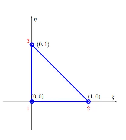
For above unit triangular element, shape function can be defined as follows.

S_1 = 1-\xi-\eta

S_2 = \xi

S_3 = \eta

Quadrilateral Element

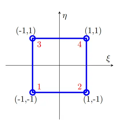
For above unit Quadrilateral element, shape function can be defined as follows.

S_1 = \frac{1}{4}(1-\xi)(1-\eta)

S_2 = \frac{1}{4}(1+\xi)(1-\eta)

S_3 = \frac{1}{4}(1+\xi)(1+\eta)

S_4 = \frac{1}{4}(1-\xi)(1+\eta)

In addition that, inverse jacobian matrix and determinant equations as follows. All of these definitions are enough to find derivatives of shape functions. General derivations are so long, and not that much essential. In the example, procedure will be shown clearly.

|J| = J_{11}J_{22}-J_{12}J_{21}

J^{-1}=\frac{1}{|J|}\begin{bmatrix} J_{22} & -J_{12} \\ -J_{21} & J_{11} \end{bmatrix}

Elemental Matrices

The difference in shape functions between triangular and quadrilateral elements was mentioned in the previous section. In this section, where necessary, this difference will be elaborated upon. Generally speaking, the difference lies in determining the limits of integration, as discussed in the Gauss quadrature section, and in the size of the elemental matrix 3×3 for triangular elements and 4×4 for quadrilateral elements reflecting the number of nodes. This difference is expected since the matrix is determined based on the number of nodes. Additionally, the differences between shapes explain variations in defining the integration limits. These aspects will be demonstrated in this section. The complexity of the operations necessitates explaining how these processes are carried out theoretically. Expressing equations without numerical values would require extensive space. Let’s begin with the elemental stiffness matrix.

Elemental Stiffness Matrix

The matrix obtained during the weak formulation is as follows:

K_{i,j}^e=\int^{}_{\Omega}\left(\frac{\partial S_i}{\partial x}k_x\frac{\partial S_j}{\partial x}+\frac{\partial S_i}{\partial y}k_y\frac{\partial S_j}{\partial y}\right)d\Omega

After obtaining the Jacobian matrix and the derivative expressions of the shape functions, and specifying the boundaries of the element, the integral is formulated as follows. Upon evaluating this integral, we obtain the elemental stiffness matrix.

d\Omega = dx \cdot dy = |J|\cdot d\xi \cdot d\eta

K_{i,j}^e=\int^{}_{\Omega}\left(\frac{\partial S_i}{\partial x}k_x\frac{\partial S_j}{\partial x}+\frac{\partial S_i}{\partial y}k_y\frac{\partial S_j}{\partial y}\right)|J|\cdot d\xi \cdot d\eta

However, as previously mentioned, this section varies according to the geometry defined in the mapping process. Below are the boundaries for triangular and quad elements, respectively.

K_{i,j}^e=\int^{1}_{-1}\int^{1}_{-1}\left(\frac{\partial S_i}{\partial x}k_x\frac{\partial S_j}{\partial x}+\frac{\partial S_i}{\partial y}k_y\frac{\partial S_j}{\partial y}\right)|J|\cdot d\xi \cdot d\eta

K_{i,j}^e=\int^{1}_{0}\int^{1-\xi}_{0}\left(\frac{\partial S_i}{\partial x}k_x\frac{\partial S_j}{\partial x}+\frac{\partial S_i}{\partial y}k_y\frac{\partial S_j}{\partial y}\right)|J|\cdot d\xi \cdot d\eta

How the 2D Gauss quadrature is performed and the differences between triangular and quad elements will be provided in the next section. Below, the constructed form of the elemental matrix and the assembly process are given. Additionally, it is crucial to note that because the shape functions are defined counterclockwise, the nodes in the element must also be defined in this direction. Otherwise, incorrect results will be obtained.

K^e = \begin{bmatrix} K_{1,1} &K_{1,2}&K_{1,3}\\ K_{2,1} &K_{2,2}&K_{2,3}\\ K_{3,1} &K_{3,2}&K_{3,3} \end{bmatrix}

K = \begin{bmatrix} K_{1,1}^1 & K_{1,3}^1& K_{1,2}^1& 0\\ K_{2,1}^1&K_{2,3}^1+K_{1,3}^2 & K_{2,2}^1+K_{1,1}^2&K_{1,2}^2\\ K_{3,1}^1&K_{3,3}^1+K_{2,3}^2 & K_{3,2}^1+K_{2,1}^2&K_{2,2}^2\\ 0&K_{3,3}^2&K_{3,1}^2&K_{3,2}^2 \end{bmatrix}

Elemental Force Vector

Creating and assembling the elemental force vector is completed through a process quite similar to that of the stiffness matrix. Below, you can see the previously defined force vector. However, similar to the stiffness matrix, the integral ranges will vary according to the geometric structure of the master element. Therefore, force vectors for triangular and quadrilateral elements are provided sequentially. Following that, a global vector view illustrating the assembly process is presented.

F_{i}^e=\int^{}_{\Omega}\left(S_i\cdot s\right)d\Omega

F_{i}^e=\int^{1}_{0}\int^{1-\xi}_{0}\left(S_i\cdot s\right)d\Omega

F_{i}^e=\int^{1}_{-1}\int^{1}_{-1}\left(S_i\cdot s\right)d\Omega

F^e =\begin{bmatrix} \int^{1}_{-1}\int^{1}_{-1} S_1\cdot s|J|d\eta d\xi\\ \int^{1}_{-1}\int^{1}_{-1} S_2\cdot s|J|d\eta d\xi\\ \int^{1}_{-1}\int^{1}_{-1} S_3\cdot s|J|d\eta d\xi \end{bmatrix}= \begin{bmatrix} F_1^e\\ F_2^e\\ F_3^e \end{bmatrix}

F = \begin{bmatrix} F_1^1\\ F_3^1+F_2^2\\ F_2^1+F_1^2\\ F_3^2 \end{bmatrix}

We have now obtained the global force vector after the assembly process. However, there is still a question about how to solve Gauss quadrature for 2D elements. We will address this topic in the next section.

Gauss Quadrature

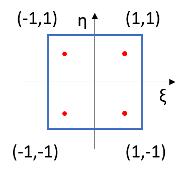
To enable the computer to solve integrals, we need a numerical integration method. Gauss quadrature is preferred as a powerful and easy numerical method commonly used in FEM solutions. It calculates various points within the element and sums them according to weight values. This method was also explained for 1D, but there are some differences because it is now applied to a plane. The following equation demonstrates how 2D Gauss quadrature is performed.

\int_{-1}^1\int_{-1}^1 f(x,y)dxdy = \sum_{j=1}^n\sum_{i=1}^n w_iw_j f(x_i,y_j)

The data points we use for the integral above are the same as in 1D. However, in 2D, we need to perform two summations. This means summing over 4 points if using 2 points and 9 points if using 3 points. Below, you can see the required table.

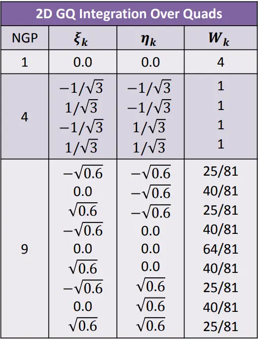
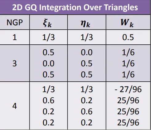
To use Gauss quadrature, the integral range must be between -1 and 1. However, this is not valid for triangular elements, as seen in the steps above. Therefore, the chosen points and weight values need to be updated accordingly. Below, you can find the relevant table and the definition of Gauss quadrature.

\int_{0}^{1}\int_{0}^{1-y} f(x,y)dxdy = \sum_{j=1}^n\sum_{i=1}^n w_iw_j f(x_i,y_j)

Boundary Conditions

Derivations for Boundary Conditions

In order to matrix equation is solvable (unique), we need boundary conditions. We should define boundary conditions for outer meshes because inner meshes are not boundary. Shape function is one for its assigned node otherwise it will be zero. This will be used. Elemental boundary condition vector definition is given below. Boundary condition can be defined as essential BC and natural BC. Essential type means exact value of that boundary is known. Natural BC means derivation term is known. Essential type just need a manipulation on our global matrix. In applying boundary condition part it will be shown. However, natural type needs derivations from given equation. Note that, for inner nodes this term will be zero. Because, it is not boundary obviously.

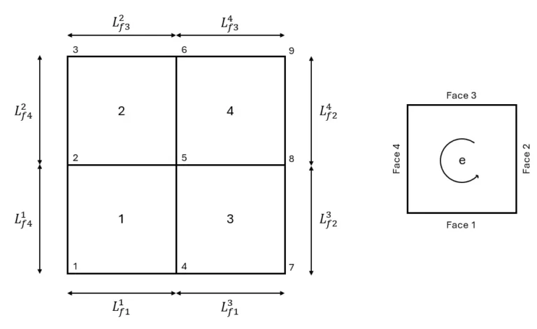
Q_{i}^e=\oint_{\Gamma}\left(S_i\cdot k_x\frac{\partial u}{\partial x}n_x+S_i\cdot k_y\frac{\partial u}{\partial y}n_y \right) d\Gamma

In order to continue derivations we need to define a reference element shape. Square shape is defined for this purpose. It is given. Global BC vector is obtained as follows.

Q = \begin{bmatrix} Q_1^1\\ Q_4^1+Q_1^2\\ Q_4^2\\ Q_2^1+Q_1^3\\ Q_3^1+Q_2^2+Q_4^3+Q_1^4\\ Q_3^2+Q_4^4\\ Q_2^3\\ Q_3^3+Q_2^4\\ Q_3^4 \end{bmatrix}=\begin{bmatrix} Q_1^1\\ Q_4^1+Q_1^2\\ Q_4^2\\ Q_2^1+Q_1^3\\ 0\\ Q_3^2+Q_4^4\\ Q_2^3\\ Q_3^3+Q_2^4\\ Q_3^4 \end{bmatrix}

Instead of calculating all the results individually, I will now demonstrate the process from this point forward. We previously noted that the inner node of the 5th element is 0, so we have taken it as such directly. We still need to compute the remaining integral values. Below is the expanded form of the integral expression. The derivative expression is given directly, based on the assumption that $q$ has a different value for each surface.

Q_{i}^e=\int_{f1}\left(S_i\cdot q_n \right) ds+\int_{f2}\left(S_i\cdot q_n \right) ds+\int_{f3}\left(S_i\cdot q_n \right) ds+\int_{f4}\left(S_i\cdot q_n \right) ds

Let’s calculate boundary condition terms for first element. Note that, q terms are labeled according to which side it is (Right, Left, Upper, Bottom).

Q_{1}^1=\int_{f1}\left(S_1\cdot q_B \right) ds+\int_{f2}\left(S_1\cdot q_n \right) ds+\int_{f3}\left(S_1\cdot q_n \right) ds+\int_{f4}\left(S_1\cdot q_L \right) ds

Face 2 and Face 3 are inner faces. Therefore, integral terms will be zero. Also, we know face lengths and shape function is linear for these boundary. That means it is triangular area shape.

Q_{1}^1=\int_{f1}\left(S_1\cdot q_B \right) ds+\int_{f4}\left(S_1\cdot q_L \right) ds

Q_{1}^1=\frac{L_{f1}^1\cdot q_B}{2} +\frac{L_{f4}^1\cdot q_L}{2}

Now, we will do similar procedure for second shape function. For this element, second node is 4th node of global shape. Again, second and third faces are inner faces. All of others, it will be same.

Q_{2}^1=\int_{f1}\left(S_2\cdot q_B \right) ds+\int_{f4}\left(S_2\cdot q_L \right) ds

Second shape function is zero throughout for face 4. Then, we obtain:

Q_{2}^1=\frac{L_{f1}^1\cdot q_B}{2}

Last node is 2nd node of global shape. We don’t need 3th one because of it is indicated as zero already when writing BC vector. Fourth shape function is zero for first face and zero for inner faces. As a result, following equation is obtained.

Q_{4}^1=\frac{L_{f4}^1\cdot q_L}{2}

Other elements can be done with same procedure. Here, it is important that know difference between global node name and elemental node name. Inner node name is start from one for each element. In addition numbering CCW. Boundary condition vector is obtained at the end of this part.

Applying Boundary Conditions

For normal BC, we should use above equation and start matrix calculation. However, if there is any essential type BC exist, then some modifications on RHS vector and LHS matrix should be applied. LHS matrix means stiffness matrix, RHS vector is sum of force and Boundary condition vector. At below, this process is shown. As expected, RHS matrix associated to that element equal to exact value, and associated value at LHS is 1 and others are 0. Equation give below helps to understand this procedure.

Q + F = \begin{bmatrix} T_1 \\ T_2 \\ \vdots\\ F_m \\ \vdots \\ T_k \\ \vdots \\ T_N \end{bmatrix}

K = \begin{bmatrix} 1 & 0 & \cdots&0& \cdots & 0& \cdots&0 \\ 0 & 1 & \cdots&0& \cdots & 0& \cdots &0 \\ \vdots &\vdots&\ddots&\vdots& \ddots & \vdots& \ddots &\vdots\\ K_{m,1} & K_{m,2} &\cdots & K_{m,m} & \cdots & K_{m,k}& \cdots &K_{m,N} \\ \vdots & \vdots &\ddots & \vdots & \ddots & \vdots& \ddots &\vdots \\ 0 & 0 & \cdots & 0 & \cdots & 1 & \cdots&0\\ \vdots& \vdots & \ddots & \vdots & \ddots & \vdots & \ddots &\vdots\\ 0 & 0 & \cdots&0& \cdots & 0& \cdots&1 \\ \end{bmatrix}

Solving Matrix Equation

The matrix equation can be expressed as above for two-side essential boundary conditions. At this point, we should solve the matrix equation. Gauss elimination is one option; however, as you can see, our matrix is diagonal, making Gauss elimination inefficient for memory and response speed. The Thomas algorithm is a better choice here, as it provides a fast response. Additionally, using a sparse matrix to construct the matrix is a good option. With sparse matrices, zeros are not stored, which positively affects memory usage. Details of these methods will not be covered in this post; this is just an advice note.

Conclusion

With this blog post, we have expanded the foundation we laid in the previous post to higher dimensions. Additionally, the Jacobian matrix was introduced, and details for quadrilateral and triangular elements were covered. Gauss Quadrature was discussed, and the application of boundary conditions was expanded. You can access solved problems for this topic through the link below. Additionally, if you review my FEM project, you will find three different examples for 2D and one example for 3D, which I believe will help you understand better. As for the assignments I prepared, both solve the same problem with different boundary conditions. In the first problem, the solution was prepared with MATLAB, while in the second problem, the solution was obtained using deal.ii. Initially, an example solution was planned for this post, but due to the length, it has been moved to another post.